Quantum Deep Dive
Solving Travelling Salesman Problem using Quantum Circuits
Quantum Deep Dive Project Submission
I chose the Quantum Deep Dive as a direction for my final project in the two semester-long Introduction to Quantum Computing Course offered by Qubit by Qubit and IBM. It involved doing some research work, implementing some research paper in the domain of Quantum Computing. This is my final project.
Abstract
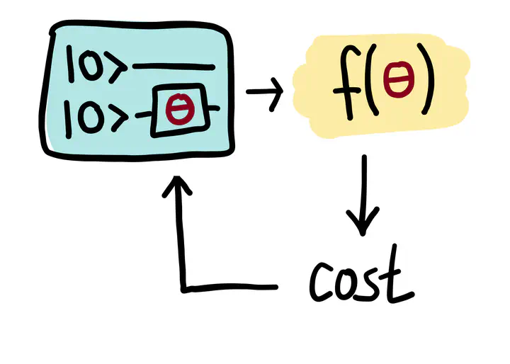
The Variational Quantum Eigensolver (VQE) algorithm is utilizes current limited quantum devices effectively and they requires a quantum circuit with parameters, called a parameterized quantum circuit (PQC), to prepare a quantum state, and the quantum state is used to calculate the expectation value of a given Hamiltonian. Here, I implement one such problem specific PQC to solve the travelling salesman problem which is discussed in the paper by Matsuo, A., Suzuki, Y., & Yamashita, S. Problem-specific parameterized quantum circuits of the VQE algorithm for optimization problems. 2020.
Table of Contents
- Formulating the Traveling Salesman Problem
- create a graph to represent our configuration
- convert the problem into a QUBO and obtain the equivalent Ising Hamiltonian
- Implementing a Problem Specific Parameterized Quantum Circuit for TSP
- construct a 3-qubit W-State with two parameters
- construct a Sampler routine
- build up a TSP entangler routine for a general case
- build up a VQE routine for the TSP entangler
- build up a Sampler routine with the optimal circuit and the list of parameter values
- build up a circuit to accomodate all the constraints
- find a TSP solution for a 4 node graph problem
- Conclusion
- Bibliography
- Reflection Questions
Formulating the Traveling Salesman Problem
This problem derives its importance from its “hardness” and ubiquitous equivalence to other relevant combinatorial optimization problems that arise in practice.
The mathematical formulation with some early analysis was proposed by W.R. Hamilton in the early 19th century. Mathematically the problem is, as in the case of Max-Cut [1], best abstracted in terms of graphs. The TSP on the nodes of a graph asks for the shortest Hamiltonian cycle that can be taken through each of the nodes. A Hamilton cycle is a closed path that uses every vertex of a graph once. The general solution is unknown and an algorithm that finds it efficiently (e.g., in polynomial time) is not expected to exist.
Find the shortest Hamiltonian cycle in a graph $G=(V,E)$ with $n=|V|$ nodes and distances, $w_{ij}$ (distance from vertex $i$ to vertex $j$). A Hamiltonian cycle is described by $N^2$ variables $x_{i,p}$, where $i$ represents the node and $p$ represents its order in a prospective cycle. The decision variable takes the value 1 if the solution occurs at node $i$ at time order $p$. We require that every node can only appear once in the cycle, and for each time a node has to occur. This amounts to the two constraints (here and in the following, whenever not specified, the summands run over 0,1,…N-1)
$$ \begin{equation}\tag{1} \sum_{i} x_{i,p} = 1 ~~\forall p. \end{equation} $$ $$ \begin{equation}\tag{2} \sum_{p} x_{i,p} = 1 ~~\forall i. \end{equation} $$
$p$ is the (discrete) time (mentioned as order here) when the $i^{th}$ node occurs. It is denoted by $x_{i,p}$.
For nodes in our prospective ordering, if $x_{i,p}$ and $x_{j,p+1}$ are both 1, then there should be an energy penalty if $(i,j) \notin E$ (not connected in the graph). The form of this penalty is
$$\sum_{i,j\notin E}\sum_{p} x_{i,p}x_{j,p+1}>0,$$
where it is assumed the boundary condition of the Hamiltonian cycles $(p=N)\equiv (p=0)$. However, here it will be assumed a fully connected graph and not include this term. The distance that needs to be minimized is
$$B(\textbf{x})=\sum_{i,j}w_{ij}\sum_{p} x_{i,p}x_{j,p+1}$$
Putting this all together in a single objective function to be minimized, we get the following:
$$C(\textbf{x})=B(\textbf{x})+ A\sum_p\left(1- \sum_i x_{i,p}\right)^2 +A\sum_i\left(1- \sum_p x_{i,p}\right)^2,$$
where $A$ is a free parameter. One needs to ensure that $A$ is large enough so that these constraints are respected. One way to do this is to choose $A$ such that $A > \mathrm{max}(w_{ij})$.
Once again, it is easy to map the problem in this form to a quantum computer, and the solution will be found by minimizing an Ising Hamiltonian. [2]
Import necessary libraries and packages
from itertools import permutations
import matplotlib.axes as axes
import matplotlib.pyplot as plt
import networkx as nx
import numpy as np
from typing import Optional

# import all necessary qiskit packages
from qiskit.algorithms import MinimumEigensolver, NumPyMinimumEigensolver, VQE
from qiskit.algorithms.minimum_eigensolvers import QAOA, SamplingVQE
from qiskit.algorithms.optimizers import L_BFGS_B, SLSQP, SPSA
from qiskit.circuit.library import TwoLocal
from qiskit.tools.visualization import plot_histogram
from qiskit.utils import algorithm_globals, QuantumInstance

from qiskit_aer import Aer

from qiskit_optimization.algorithms import MinimumEigenOptimizer
from qiskit_optimization.applications import Maxcut, Tsp
from qiskit_optimization.problems import QuadraticProgram
<frozen importlib._bootstrap>:219: RuntimeWarning: scipy._lib.messagestream.MessageStream size changed, may indicate binary incompatibility. Expected 56 from C header, got 64 from PyObject
Create helper functions
# Draw and visualize graph solution
def draw_graph(G, colors, pos):
    default_axes = plt.axes(frameon=True)
    nx.draw_networkx(G, node_color=colors, node_size=900, alpha=0.9, ax=default_axes, pos=pos, node_shape="o")
    edge_labels = nx.get_edge_attributes(G, "weight")
    nx.draw_networkx_edge_labels(G, pos=pos, edge_labels=edge_labels)
# Compute cost of the obtained result and display result
def TSPCost(energy, result_bitstring, adj_matrix):
    print("-------------------")
    print("Energy:", energy)
    print("Tsp objective:", energy + offset)
    print("Feasibility:", qubo.is_feasible(result_bitstring))

    solution_vector = tsp.interpret(result_bitstring)
    print("Solution Vector:", solution_vector)
    print("Solution Objective:", tsp.tsp_value(solution_vector, adj_matrix))
    print("-------------------")

    # Draw Graph
    draw_tsp_solution(tsp.graph, solution_vector, colors, pos)
# Plots a convergence graph
def PlotGraph(ideal, mean):
    plt.figure(figsize=(8, 6))
    # Plot label
    for value in range(len(mean)):
        plt.plot(mean[value], label="Proposal {}".format(value+1) )

    # Ideal plot
    plt.axhline(y=ideal, color="tab:red", ls="--", label="Target")
    plt.legend(loc="best")
    plt.xlabel("Optimizer iteration")
    plt.ylabel("Energy")

    # Plot graph title
    plt.title("TSP Entangler Line {} Constraint".format(len(mean)))
    plt.show()
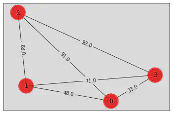
Let’s represent our graph.
# Let us first generate a graph with 4 nodes!

n = 4
num_qubits = 4 ** 2

tsp = Tsp.create_random_instance(n, seed=123)
adj_matrix = nx.to_numpy_matrix(tsp.graph)
print("distance\n", adj_matrix)

colors = ["r" for node in tsp.graph.nodes]
pos = [tsp.graph.nodes[node]["pos"] for node in tsp.graph.nodes]
draw_graph(tsp.graph, colors, pos)
distance
 [[ 0. 48. 91. 33.]
 [48.  0. 63. 71.]
 [91. 63.  0. 92.]
 [33. 71. 92.  0.]]
Brute force approach
The brute force approach involves trying every combination through classical computation to find the optimal solution. As we can infer, this procedure becomes more computationally-intensive as the number of nodes increases, or as the number of locations the traveling salesman must visit, increases.
from itertools import permutations
def brute_force_tsp(w, N):
a = list(permutations(range(1, N)))
last_best_distance = 1e10
for i in a:
distance = 0
pre_j = 0
for j in i:
distance = distance + w[j, pre_j]
pre_j = j
distance = distance + w[pre_j, 0]
order = (0,) + i
if distance < last_best_distance:
best_order = order
last_best_distance = distance
print("order = " + str(order) + " Distance = " + str(distance))
return last_best_distance, best_order
best_distance, best_order = brute_force_tsp(adj_matrix, n)
print(
"Best order from brute force = "
+ str(best_order)
+ " with total distance = "
+ str(best_distance)
)
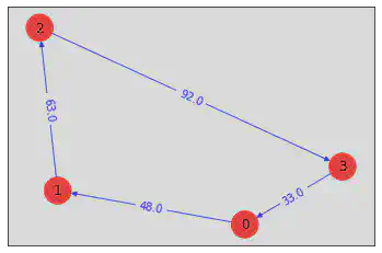
def draw_tsp_solution(G, order, colors, pos):
G2 = nx.DiGraph()
G2.add_nodes_from(G)
n = len(order)
for i in range(n):
j = (i + 1) % n
G2.add_edge(order[i], order[j], weight=G[order[i]][order[j]]["weight"])
default_axes = plt.axes(frameon=True)
nx.draw_networkx(
G2, node_color=colors, edge_color="b", node_size=600, alpha=0.8, ax=default_axes, pos=pos
)
edge_labels = nx.get_edge_attributes(G2, "weight")
nx.draw_networkx_edge_labels(G2, pos, font_color="b", edge_labels=edge_labels)
draw_tsp_solution(tsp.graph, best_order, colors, pos)
order = (0, 1, 2, 3) Distance = 236.0
Best order from brute force = (0, 1, 2, 3) with total distance = 236.0

Examine the quantum approach
1. Call the TSP Application Class and create a Quadratic Program instance
To solve this optimization problem, we first need to convert the TSP problem into a quadratic program, a program which lays out the optimization problem as a quadratic objective function and relevant constraint functions. The TSP defines variables as binary variables, so we will see those defined in the quadratic program as well.
qp = tsp.to_quadratic_program()
print(qp.prettyprint())
Problem name: TSP

Minimize
  48*x_0_0*x_1_1 + 48*x_0_0*x_1_3 + 91*x_0_0*x_2_1 + 91*x_0_0*x_2_3
  + 33*x_0_0*x_3_1 + 33*x_0_0*x_3_3 + 48*x_0_1*x_1_0 + 48*x_0_1*x_1_2
  + 91*x_0_1*x_2_0 + 91*x_0_1*x_2_2 + 33*x_0_1*x_3_0 + 33*x_0_1*x_3_2
  + 48*x_0_2*x_1_1 + 48*x_0_2*x_1_3 + 91*x_0_2*x_2_1 + 91*x_0_2*x_2_3
  + 33*x_0_2*x_3_1 + 33*x_0_2*x_3_3 + 48*x_0_3*x_1_0 + 48*x_0_3*x_1_2
  + 91*x_0_3*x_2_0 + 91*x_0_3*x_2_2 + 33*x_0_3*x_3_0 + 33*x_0_3*x_3_2
  + 63*x_1_0*x_2_1 + 63*x_1_0*x_2_3 + 71*x_1_0*x_3_1 + 71*x_1_0*x_3_3
  + 63*x_1_1*x_2_0 + 63*x_1_1*x_2_2 + 71*x_1_1*x_3_0 + 71*x_1_1*x_3_2
  + 63*x_1_2*x_2_1 + 63*x_1_2*x_2_3 + 71*x_1_2*x_3_1 + 71*x_1_2*x_3_3
  + 63*x_1_3*x_2_0 + 63*x_1_3*x_2_2 + 71*x_1_3*x_3_0 + 71*x_1_3*x_3_2
  + 92*x_2_0*x_3_1 + 92*x_2_0*x_3_3 + 92*x_2_1*x_3_0 + 92*x_2_1*x_3_2
  + 92*x_2_2*x_3_1 + 92*x_2_2*x_3_3 + 92*x_2_3*x_3_0 + 92*x_2_3*x_3_2

Subject to
  Linear constraints (8)
    x_0_0 + x_0_1 + x_0_2 + x_0_3 == 1  'c0'
    x_1_0 + x_1_1 + x_1_2 + x_1_3 == 1  'c1'
    x_2_0 + x_2_1 + x_2_2 + x_2_3 == 1  'c2'
    x_3_0 + x_3_1 + x_3_2 + x_3_3 == 1  'c3'
    x_0_0 + x_1_0 + x_2_0 + x_3_0 == 1  'c4'
    x_0_1 + x_1_1 + x_2_1 + x_3_1 == 1  'c5'
    x_0_2 + x_1_2 + x_2_2 + x_3_2 == 1  'c6'
    x_0_3 + x_1_3 + x_2_3 + x_3_3 == 1  'c7'

  Binary variables (16)
    x_0_0 x_0_1 x_0_2 x_0_3 x_1_0 x_1_1 x_1_2 x_1_3 x_2_0 x_2_1 x_2_2 x_2_3
    x_3_0 x_3_1 x_3_2 x_3_3
2. Convert the quadratic program to QUBO and Ising Hamiltonian
To solve this problem, we need to convert our quadratic program into a form that a quantum computer can work with. In this case we will generate an Ising Hamiltonian, which is simply a representation (i.e. model) of the energy of this particular system (i.e. problem). We can use eigensolvers to find the minimum energy of the Ising hamiltonian, which corresponds to the shortest path and the solution of our problem.
How do we get the Ising Hamiltonian? First, we convert the quadratic program to a QUBO (Quadratic Unconstrained Binary Optimization), a combinatorial optimization problem representation to then obtain an Ising Hamiltonian.
from qiskit_optimization.converters import QuadraticProgramToQubo

qp2qubo = QuadraticProgramToQubo()   #instatiate qp to qubo class
qubo = qp2qubo.convert(qp)      # convert quadratic program to qubo
qubitOp, offset = qubo.to_ising()      #convert qubo to ising

print("Offset:", offset)
print("Ising Hamiltonian:", str(qubitOp))
Offset: 51756.0
Ising Hamiltonian: -6456.0 * IIIIIIIIIIIIIIIZ
- 6456.0 * IIIIIIIIIIIIIIZI
- 6456.0 * IIIIIIIIIIIIIZII
- 6456.0 * IIIIIIIIIIIIZIII
- 6461.0 * IIIIIIIIIIIZIIII
- 6461.0 * IIIIIIIIIIZIIIII
- 6461.0 * IIIIIIIIIZIIIIII
- 6461.0 * IIIIIIIIZIIIIIII
- 6493.0 * IIIIIIIZIIIIIIII
- 6493.0 * IIIIIIZIIIIIIIII
- 6493.0 * IIIIIZIIIIIIIIII
- 6493.0 * IIIIZIIIIIIIIIII
- 6468.0 * IIIZIIIIIIIIIIII
- 6468.0 * IIZIIIIIIIIIIIII
- 6468.0 * IZIIIIIIIIIIIIII
- 6468.0 * ZIIIIIIIIIIIIIII
+ 1592.5 * IIIIIIIIIIIIIIZZ
+ 1592.5 * IIIIIIIIIIIIIZIZ
+ 1592.5 * IIIIIIIIIIIIIZZI
+ 1592.5 * IIIIIIIIIIIIZIIZ
+ 1592.5 * IIIIIIIIIIIIZIZI
+ 1592.5 * IIIIIIIIIIIIZZII
+ 1592.5 * IIIIIIIIIIIZIIIZ
+ 12.0 * IIIIIIIIIIIZIIZI
+ 12.0 * IIIIIIIIIIIZZIII
+ 12.0 * IIIIIIIIIIZIIIIZ
+ 1592.5 * IIIIIIIIIIZIIIZI
+ 12.0 * IIIIIIIIIIZIIZII
+ 1592.5 * IIIIIIIIIIZZIIII
+ 12.0 * IIIIIIIIIZIIIIZI
+ 1592.5 * IIIIIIIIIZIIIZII
+ 12.0 * IIIIIIIIIZIIZIII
+ 1592.5 * IIIIIIIIIZIZIIII
+ 1592.5 * IIIIIIIIIZZIIIII
+ 12.0 * IIIIIIIIZIIIIIIZ
+ 12.0 * IIIIIIIIZIIIIZII
+ 1592.5 * IIIIIIIIZIIIZIII
+ 1592.5 * IIIIIIIIZIIZIIII
+ 1592.5 * IIIIIIIIZIZIIIII
+ 1592.5 * IIIIIIIIZZIIIIII
+ 1592.5 * IIIIIIIZIIIIIIIZ
+ 22.75 * IIIIIIIZIIIIIIZI
+ 22.75 * IIIIIIIZIIIIZIII
+ 1592.5 * IIIIIIIZIIIZIIII
+ 15.75 * IIIIIIIZIIZIIIII
+ 15.75 * IIIIIIIZZIIIIIII
+ 22.75 * IIIIIIZIIIIIIIIZ
+ 1592.5 * IIIIIIZIIIIIIIZI
+ 22.75 * IIIIIIZIIIIIIZII
+ 15.75 * IIIIIIZIIIIZIIII
+ 1592.5 * IIIIIIZIIIZIIIII
+ 15.75 * IIIIIIZIIZIIIIII
+ 1592.5 * IIIIIIZZIIIIIIII
+ 22.75 * IIIIIZIIIIIIIIZI
+ 1592.5 * IIIIIZIIIIIIIZII
+ 22.75 * IIIIIZIIIIIIZIII
+ 15.75 * IIIIIZIIIIZIIIII
+ 1592.5 * IIIIIZIIIZIIIIII
+ 15.75 * IIIIIZIIZIIIIIII
+ 1592.5 * IIIIIZIZIIIIIIII
+ 1592.5 * IIIIIZZIIIIIIIII
+ 22.75 * IIIIZIIIIIIIIIIZ
+ 22.75 * IIIIZIIIIIIIIZII
+ 1592.5 * IIIIZIIIIIIIZIII
+ 15.75 * IIIIZIIIIIIZIIII
+ 15.75 * IIIIZIIIIZIIIIII
+ 1592.5 * IIIIZIIIZIIIIIII
+ 1592.5 * IIIIZIIZIIIIIIII
+ 1592.5 * IIIIZIZIIIIIIIII
+ 1592.5 * IIIIZZIIIIIIIIII
+ 1592.5 * IIIZIIIIIIIIIIIZ
+ 8.25 * IIIZIIIIIIIIIIZI
+ 8.25 * IIIZIIIIIIIIZIII
+ 1592.5 * IIIZIIIIIIIZIIII
+ 17.75 * IIIZIIIIIIZIIIII
+ 17.75 * IIIZIIIIZIIIIIII
+ 1592.5 * IIIZIIIZIIIIIIII
+ 23.0 * IIIZIIZIIIIIIIII
+ 23.0 * IIIZZIIIIIIIIIII
+ 8.25 * IIZIIIIIIIIIIIIZ
+ 1592.5 * IIZIIIIIIIIIIIZI
+ 8.25 * IIZIIIIIIIIIIZII
+ 17.75 * IIZIIIIIIIIZIIII
+ 1592.5 * IIZIIIIIIIZIIIII
+ 17.75 * IIZIIIIIIZIIIIII
+ 23.0 * IIZIIIIZIIIIIIII
+ 1592.5 * IIZIIIZIIIIIIIII
+ 23.0 * IIZIIZIIIIIIIIII
+ 1592.5 * IIZZIIIIIIIIIIII
+ 8.25 * IZIIIIIIIIIIIIZI
+ 1592.5 * IZIIIIIIIIIIIZII
+ 8.25 * IZIIIIIIIIIIZIII
+ 17.75 * IZIIIIIIIIZIIIII
+ 1592.5 * IZIIIIIIIZIIIIII
+ 17.75 * IZIIIIIIZIIIIIII
+ 23.0 * IZIIIIZIIIIIIIII
+ 1592.5 * IZIIIZIIIIIIIIII
+ 23.0 * IZIIZIIIIIIIIIII
+ 1592.5 * IZIZIIIIIIIIIIII
+ 1592.5 * IZZIIIIIIIIIIIII
+ 8.25 * ZIIIIIIIIIIIIIIZ
+ 8.25 * ZIIIIIIIIIIIIZII
+ 1592.5 * ZIIIIIIIIIIIZIII
+ 17.75 * ZIIIIIIIIIIZIIII
+ 17.75 * ZIIIIIIIIZIIIIII
+ 1592.5 * ZIIIIIIIZIIIIIII
+ 23.0 * ZIIIIIIZIIIIIIII
+ 23.0 * ZIIIIZIIIIIIIIII
+ 1592.5 * ZIIIZIIIIIIIIIII
+ 1592.5 * ZIIZIIIIIIIIIIII
+ 1592.5 * ZIZIIIIIIIIIIIII
+ 1592.5 * ZZIIIIIIIIIIIIII
Using NumPyMinimumEigensolver to obtain a reference solution
# Making the Hamiltonian in its full form and getting the lowest eigenvalue and eigenvector
ee = NumPyMinimumEigensolver()
result = ee.compute_minimum_eigenvalue(qubitOp)

energy_numpy = result.eigenvalue.real
# Call helper function to compute cost of the obtained result and display result
TSPCost(energy = result.eigenvalue.real, result_bitstring = tsp.sample_most_likely(result.eigenstate), adj_matrix = adj_matrix)
-------------------
Energy: -51520.0
Tsp objective: 236.0
Feasibility: True
Solution Vector: [1, 2, 3, 0]
Solution Objective: 236.0
-------------------
3. Running it on a quantum computer
I have presented the results of the quantum computer’s computation below.
VQE Routine Not Converging Well
When running the same problem earlier. The results can be slightly different from when we run the same problem due to the heuristic nature of the algorithm, but we can see that it is not showing good convergence to the solution. The ‘solution objective’ (solution of our objective function) gave us ‘302.0,’ which is higher than our reference solution (shortest path) ‘236.0.’
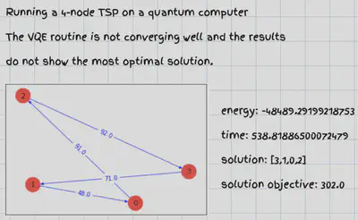
Note: The above is provided since the actual computation on the quantum computer takes a long time to finish.
Heuristic Algorithms
In many applications it is important to find the minimum eigenvalue of a matrix. For example, in chemistry, the minimum eigenvalue of a Hermitian matrix characterizing the molecule is the ground state energy of that system. As we learned earlier, we can map our shortest path problem into an Ising Hamiltonian, which allows us to search for the shortest path in the same way we find the ground state energy of a molecule.
We may have heard that a quantum state can be represented as a vector in a complex vector space. This space where all the possible quantum states exist is mathematically called a ‘Hilbert Space.’ As the optimization problem grows in size and the more number of constraints we need to take into consideration, this adds a degree of complexity that will grow our Hilbert Space exponentially.
Problems like the Traveling Salesman Problem are known to be NP-Hard due to how our solution space grows exponentially with each city and constraints added.
This ‘NP-hardness’ in theoretical computer science make heuristics the only viable option for a variety of complex optimization problems that need to be routinely solved in real-world applications where the objective of a heuristic approach is to produce a solution in a reasonable time frame that is good enough for solving the problem at hand. This solution may not be the best of all the solutions to this problem, or it may simply approximate the exact solution. But it is still valuable because finding it does not require a prohibitively long time.
We may realize that this indicates that there is a ’trade-off’ between optimality and execution time. Some heuristics converge faster than others. How can we get better convergence with our current quantum systems with limited number of qubits? Now, we will explore this notion by looking at an approach that can help reduce our search space so we can arrive at a good solution in a relatively reasonable amount of time.
Need for a problem-specific parameterized quantum circuit (PQC)
The “natural form” of a QUBO model inherently is an unconstrained problem, other than those requiring the variables to be binary (hence the name Quadratic Unconstrained Binary Optimization). Most of the problems that are of interest to mankind tend to include additional constraints in the formulation of the problem to obtain good solutions. Many of these constrained models can be effectively re-formulated as a QUBO model by introducing penalties into the objective function as an alternative to explicitly imposing constraints to best fit the problem construction. [3]
We can utilize the constraints of our TSP problem to dynamically construct a problem-specific PQC that reflects those constraints of the optimization problem. Therefore, we can restrict a unitary transformation that is provided by the problem-specific PQC while taking constraints into account. This makes it possible to make the search space smaller in hopes of arriving at an optimal or near-optimal solution!
Implementing a Problem Specific Parameterized Quantum Circuit for TSP
As mentioned above, we shall be looking at implementing a problem specific PQC for our TSP problem to attempt to reduce our search space and arrive at a good solution. This is an active area of interest and there are multiple PQC approaches for the TSP problem, however specifically, we shall be looking at one of the implementations by Matsuo, A., Suzuki, Y., & Yamashita, S. Problem-specific parameterized quantum circuits of the VQE algorithm for optimization problems. 2020. [4]
One of the reasons of intractability for many problems comes from the huge search space that exists for a solution. With so many possibilities to evaluate, a brute force search approach quickly becomes computationally unfeasible. The idea here is to reduce the subspace in such a way that it still includes the solution subspace, but is significantly smaller than the complete subspace, lets call it $|S_{all}|$. So the main objective is to propose a PQC that gives us a subspace: $S_{proposed}$ that includes $S_{feasible_solutions}$, but such that the size of $S_{proposed}$ subspace is smaller than $|S_{all}|$. This increases the possibility of arriving at optimal or near optimal solution while reducing the required time to find the same as compared to, let’s say, using a heuristic approach on the whole subspace!
Usually, an optimization problem can have more than one constraint. For such cases, we create multiple problem-specific parameterized quantum sub-circuits, each of which reflect the corresponding constraint. Then, by combining those sub-circuits properly, even though the optimization problem has more than one constraint, it is still possible to create a problem-specific PQC and reduce the search space.
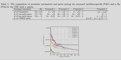
The paper we mentioned above proposes 4 different types of PQCs approaching the problem in different ways, each with different characteristics and constraints considered. For the NISQ era, characteristics of a circuit such as number of gates, parameters, entanglement and circuit depth are important factors when designing PQCs and here we shall be looking into a few of the approaches as showcased in the paper above. We will be utilizing the VQE algorithm to build upon the routine to get our results using the Estimator and Sampler primitive!
PQCs satisfying only the constraints on the first line Eq. (1)
Let’s check out the first type of problem-specific PQC as proposed for our TSP problem here to effectively collect our space debris. The paper proposes us to take into account only the constraints in the first line as shown below:
$$\sum_{i}^{N} x_{i,p} = 1 ~~\forall p = 1…N.$$
As we can see, in each of the constraints, exactly one of the variables has to be one while the other variables have to be zero. This type of constraint restricts the set of solutions to the set of bases corresponding to the $W$ state.
A $W$ state is a superposition of states where exactly one of the qubits is $|1\rangle$ while all other qubits are $|0\rangle$ with equal amplitudes. A $W$ state for $n$ qubits is represented as $|W\rangle = \frac{1}{\sqrt{2^n}} (|10…0\rangle + |01…0\rangle + |00…1\rangle)$. Each of the bases of this state corresponds to the constraint as mentioned above $\sum{x_i} = 1$. Since the other bases do not satisfy the constraint of $\sum{x_i} = 1$, we do not consider them here hence reducing our subspace for solving the problem with considerations of the constraints from the equation in the first line. We shall create circuits representing the $W$ state in such a way that we can control the amplitudes of each base.
$$|W(φ)\rangle = \sum_{i} α_{i(φ)}|ψ_i\rangle, $$ $$\sum_{i} {|α_{i(φ)}|}^2 = 1, $$ $$|ψ_i\rangle ∈ {{|10…0\rangle, |01…0\rangle, |00…1\rangle}}$$
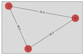
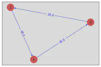
Let us see how we can do that for a 3 qubit example.
# Define 3 Node graph
n = 3
num_qubits = n**2
tsp = Tsp.create_random_instance(n, seed=250)

adj_matrix = nx.to_numpy_matrix(tsp.graph)

# Plot graph
colors = ["tab:red" for node in tsp.graph.nodes]
pos = [tsp.graph.nodes[node]["pos"] for node in tsp.graph.nodes]

print("Learning problem 3 Node graph: ")
draw_graph(tsp.graph, colors, pos)

# Define quadratic program for 4 node graph
qp = tsp.to_quadratic_program()

# Define Ising operator for 3 Node graph
qp2qubo = QuadraticProgramToQubo()
qubo = qp2qubo.convert(qp)
qubitOp, offset = qubo.to_ising()

# Making the Hamiltonian in its full form and getting the lowest eigenvalue and eigenvector
ee = NumPyMinimumEigensolver()
result = ee.compute_minimum_eigenvalue(qubitOp)

# Ideal result
ideal = result.eigenvalue.real
print(f"Ideal energy: {ideal}")
Learning problem 3 Node graph:
Ideal energy: -4751.0
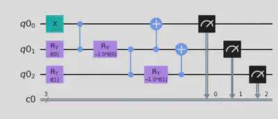
from qiskit import QuantumRegister, ClassicalRegister
from qiskit.circuit import ParameterVector, QuantumCircuit
# Initialize circuit
qr = QuantumRegister(3)
cr = ClassicalRegister(3)
circuit = QuantumCircuit(qr,cr)
# Initialize Parameter with θ
theta = ParameterVector('θ', 2)
# Apply gates to circuit
circuit.x(0)
circuit.ry(theta[0], 1)
circuit.cz(0, 1)
circuit.ry(-theta[0], 1)
circuit.ry(theta[1], 2)
circuit.cz(1, 2)
circuit.ry(-theta[1], 2)
circuit.cx(1, 0)
circuit.cx(2, 1)
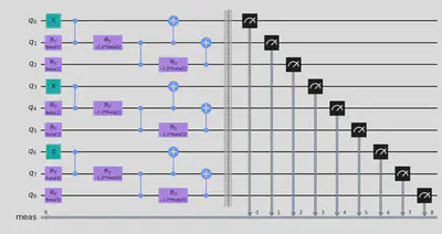
circuit.measure(qr,cr)
circuit.draw("mpl")
Running it on the Sampler primitive
Now we run the circuit with some parameters and observe the quasi-probability distribution! As per the paper we should be seeing the probability distribution being controlled as per the equation (11) in section 3.2.1 in the paper.
$$α_{1(φ)} |100\rangle + α_{2(φ)} |010\rangle + α_{3(φ)} |001\rangle,$$ $$\sum_{i}^3 {|α_{i(φ)}|}^2 = 1, $$ $$α_{1(φ)} = cos(\theta_1), α_{2(φ)} = -sin(\theta_1) cos(\theta_2), α_{3(φ)} = sin(\theta_1) sin(\theta_2)$$
For an example’s sake, let’s try to get an equal distribution for the 3 qubit state. That would mean we should be seeing equal/near equal distributions for the states $|100\rangle, |010\rangle, |001\rangle$ i.e. decimal states $1, 2 $ and $4$ if we satisfy the equation above to have $α_{1(φ)} = α_{2(φ)} = α_{3(φ)}$
Let us visualize and confirm this result! According to the equation above, solving it to see a near equal probability across the three states of 1, 2 and 4, we can enter in $\theta_1$ as 54.73 degrees and $\theta_2$ as 45 degrees!
from qiskit_ibm_runtime import QiskitRuntimeService

# Initialize service and backend
#QiskitRuntimeService.save_account(channel='ibm_quantum', token='my_token', overwrite=True)

# Set simulator
backend = service.backends(simulator=True)[0]
print(backend)
<IBMBackend('ibmq_qasm_simulator')>
from math import pi
from qiskit_ibm_runtime import Session, Sampler, Options

options = Options(simulator={"seed_simulator": 42},resilience_level=0) #DO NOT CHANGE

# Define sampler object
with Session(service=service, backend=backend):
    sampler = Sampler(options=options) # Define sampler with options above
    result = sampler.run(circuits=circuit, parameter_values=[[54.73*2*np.pi/360, 45*2*np.pi/360]], shots=5000) # Run the sampler. Remember, the theta here is in degrees! :)

# Plot result
result_dict = result.result().quasi_dists[0] # Obtain the quasi distribution. Note: Expected result type: QuasiDistribution dict

values = list(result_dict.keys()) # Obtain all the values in a list
probabilities = list(result_dict.values()) # Obtain all the probabilities in a list

plt.bar(values,probabilities,tick_label=values)
plt.show()
print(result_dict)
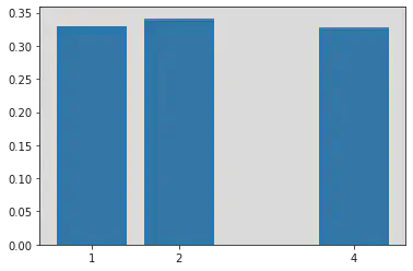
{1: 0.3298, 4: 0.3286, 2: 0.3416}
We may not see an exact distribution due to the randomness added by the simulator and the less precise theta value used here. But nonetheless, we have achieved our intended example objective!
Now let’s proceed to apply this to an algorithm and see how we can use this state for our problem as per the paper!

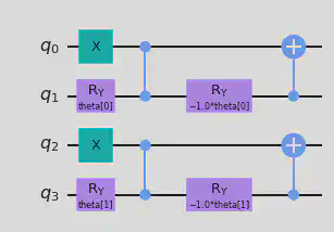
We will now proceed to build the routine as suggested above. For a TSP problem, the problem is encoded for an $N$ node graph is encoded in $N^2$ qubits. We need to append the W gate routine in this order for the PQC to be applied successfully as per our problem constraint. We will first look at a case for a 2 node graph and then proceed to have a generalized function to generate the W state for any arbitrary value of N.

For an example here, let us consider this condition for a 2 node graph. For a 2 node graph, we would require 4 qubits. Note, here we shall follow the row-major order. The first two qubits would represent the columns of the first row respectively as shown in the figure and the last 2 qubits would represent the columns in the $N^{th}$ row which in this case are the two elements in the second row. The number of parameters we require in general would be $(N)*(N-1)$. Let’s check out how to apply this TSP entangler routine for a 2 node graph and extrapolate this for the general solution.
# Two Node TSP entangler
from qiskit import QuantumRegister, ClassicalRegister
from qiskit.circuit import ParameterVector, QuantumCircuit

# Set value of N
N = 2

# Define Circuit and ParameterVector
circuit = QuantumCircuit(N**2)
theta =  ParameterVector('theta',length=(N-1)*N)

# Block 1 ----------------
# X Gate -----------------
circuit.x(0)
# Parameter Gates --------
circuit.ry(theta[0],1)
circuit.cz(0,1)
circuit.ry(-theta[0],1)
# CX gates ---------------
circuit.cx(1,0)

# Block 2 ----------------
# X Gate -----------------
circuit.x(2)
# Parameter Gates --------
circuit.ry(theta[1],3)
circuit.cz(2,3)
circuit.ry(-theta[1],3)
# CX gates ---------------
circuit.cx(3,2)

circuit.draw("mpl")
For a graph with $N = 3$, we will be following the same. The circuit we made previously will be the one that will be applied 3 times as a block. In general, we will have the W state applied for N qubits as one block. In total, there will be N blocks across $N^2$ qubits to complete the problem.
We shall build up a TSP entangler routine for the above shown constraint for any general N qubit case.
from qiskit import QuantumRegister, ClassicalRegister
from qiskit.circuit import ParameterVector, QuantumCircuit

def tsp_entangler(N):

    # Define QuantumCircuit and ParameterVector size
    circuit = QuantumCircuit(N**2)
    theta =  ParameterVector('theta',length=(N-1)*N)

    k = 0
    for i in range(N):
        # X Gate
        circuit.x(i*N)

        # Parameter Gates
        for j in range(N*i+1, N*(i+1)):
            circuit.ry(theta[k],j)
            circuit.cz(j-1,j)
            circuit.ry(-theta[k],j)
            k += 1

        # CX gates
        for j in range(N*i+1, N*(i+1)):
            circuit.cx(j, j-1)

    return circuit
We now have the building blocks to run our PQC and test our solution! Let’s start constructing the VQE function for calculating our best result for the problem. We shall be using the VQE class to build up our VQE routine and calculate the result using the Estimator Primitive.
Solving the problem using the VQE class
The VQE class in Qiskit is now refactored to leverage the Quantum primitive construct. It uses a variational technique to find the minimum eigenvalue of a given diagonal operator but is executed using the Estimator primitive.
An instance of VQE also requires an ansatz, a parameterized QuantumCircuit, to prepare the trial state $|\psi(\vec\theta)\rangle$. It also needs a classical optimizer which varies the circuit parameters $\vec\theta$ such that the expectation value of the operator on the corresponding state approaches a minimum. In this case we are interested in extracting the result bitstring corresponding to the optimal solution from the converged result.
These are the following values it takes as per the Qiskit Documentation:
Arguments:
estimator: The estimator primitive to compute the expectation value of the Hamiltonian operator.ansatz: A parameterized quantum circuit to prepare the trial state.optimizer: A classical optimizer to find the minimum energy. This can either be a Qiskit.Optimizer or a callable implementing the .Minimizer protocol.initial_point: An optional initial point (i.e. initial parameter values) for the optimizer. The length of the initial point must match the number of ansatz parameters. If None, a random point will be generated within certain parameter bounds. SamplingVQE will look to the ansatz for these bounds. If the ansatz does not specify bounds, bounds of -2\pi, 2\pi will be used.callback: A callback that can access the intermediate data at each optimization step. These data are: the evaluation count, the optimizer parameters for the ansatz, the estimated value, and the metadata dictionary.
# Imports
from qiskit_optimization import QuadraticProgram
from qiskit_optimization.algorithms import MinimumEigenOptimizer
from qiskit.algorithms.minimum_eigen_solvers import NumPyMinimumEigensolver,  MinimumEigensolver
from qiskit.algorithms.minimum_eigensolvers import SamplingVQE, VQE
from qiskit.circuit.library import TwoLocal
from qiskit.algorithms.optimizers import SPSA, SLSQP, L_BFGS_B
from qiskit.quantum_info import SparsePauliOp
from qiskit.primitives import Estimator
import numpy as np
# Define PQC for 3 node graph
PQC = tsp_entangler(3)
def RunVQE(estimator, model, optimizer, operator, init=None):

    # Store intermediate results
    history = {"eval_count": [], "parameters": [], "mean": [], "metadata": []}

    # Define callback function
    def store_intermediate_result(eval_count, parameters, mean, metadata):
        history["eval_count"].append(eval_count)
        history["parameters"].append(parameters)
        history["mean"].append(mean.real)

    # Define VQE run
    vqe = VQE(estimator=estimator, ansatz=model, optimizer=optimizer, initial_point=init, callback=store_intermediate_result)

    # Compute minimum_eigenvalue
    result = vqe.compute_minimum_eigenvalue(operator)

    return result, history["mean"]
Running the routine and checking our result for the first PQC for 3 qubit case:
%%time
from qiskit.utils import algorithm_globals
from qiskit.primitives import Estimator
algorithm_globals.random_seed = 123

# Define optimizer
optimizer = SPSA(maxiter=50)

# Define Initial point
np.random.seed(10)
init = np.random.rand((n-1)*n) * 2 * np.pi

# Define backend
backend = service.backends(simulator=True)[0]

# Call RunVQE. Do not pass in options
with Session(service = service, backend = backend):
    result, mean = RunVQE(Estimator(), PQC, optimizer, qubitOp, init)

# Print result
print(result)
{   'aux_operators_evaluated': None,
    'cost_function_evals': 100,
    'eigenvalue': -4750.85369976058,
    'optimal_circuit': <qiskit.circuit.quantumcircuit.QuantumCircuit object at 0x7fca288ae040>,
    'optimal_parameters': {   ParameterVectorElement(theta[3]): 4.70869194010299,
                              ParameterVectorElement(theta[0]): 3.1405938762891474,
                              ParameterVectorElement(theta[5]): 3.147716694624536,
                              ParameterVectorElement(theta[2]): 4.708620211338824,
                              ParameterVectorElement(theta[4]): 4.706895428144666,
                              ParameterVectorElement(theta[1]): -1.660067101003188},
    'optimal_point': array([ 3.14059388, -1.6600671 ,  4.70862021,  4.70869194,  4.70689543,
        3.14771669]),
    'optimal_value': -4750.85369976058,
    'optimizer_evals': None,
    'optimizer_result': <qiskit.algorithms.optimizers.optimizer.OptimizerResult object at 0x7fca28830a00>,
    'optimizer_time': 0.8081450462341309}
CPU times: user 794 ms, sys: 18.5 ms, total: 813 ms
Wall time: 810 ms
Computing the Eigenstate from the VQEResult object
Next here, we shall proceed to compute the Eigenstate of our solution and get our best distribution binary string from the VQEResult object. To obtain the eigenstate, we shall sample the parametrized ansatz with the optimal parameters that we obtained by running the Estimator call on our VQE function. We shall use the Sampler here to sample our ansatz with the optimal_parameters from the VQEResult object. The key corresponding to the maximum of the nearest_probability_distribution we obtain will be our binary state of the best solution which we will pass on to evaluate!
Let’s setup our Sampler routine for the same. First, we will extract the optimal_circuit from our computed result and apply measurements for the Sampler routine. Here we use inplace=False to make sure we store the circuit with measurements as a new circuit.
optimal = result.optimal_circuit.measure_all(inplace=False) # Extract optimal circuit and add measurements
optimal.draw("mpl")
Setting up Sampler to obtain our best bitstring
Next, let us proceed to setup our Sampler to obtain the best bitstring from the result we just computed. Here we shall pass the optimal circuit with the measurements as computed above and extract the optimal_parameters list from result.
A note on the usage of nearest_probability_distribution: While a Quasiprobability distribution does offer a wider gamut of information data points at our disposal, we cannot directly substitute it for a real probability distribution. For a Quasiprobability distribution to be converted into a true probability distribution, we shall use here the
nearest_probability_distribution()function. This function takes a quasiprobability distribution as an input and maps it to the closest probability distribution as defined by the L2-norm up to a certain error bound
We shall now use this to get our eigenstate and obtain the optimal result from this distribution!
list(result.optimal_parameters.values())
[3.1405938762891474,
 -1.660067101003188,
 4.708620211338824,
 4.70869194010299,
 4.706895428144666,
 3.147716694624536]
def BestBitstring(result, optimal_circuit):
    energy = result.eigenvalue.real

    options = Options(simulator={"seed_simulator": 42},resilience_level=0)

    with Session(service = service, backend = backend):
        sampler_result = Sampler(options=options).run(optimal_circuit, parameter_values=[list(result.optimal_parameters.values())]).result()

    result_prob_dist = sampler_result.quasi_dists[0].nearest_probability_distribution() # Obtain the nearest_probability_distribution for the sampler result from the quasi distribution obtained

    max_key = format(max(result_prob_dist, key = result_prob_dist.get),"016b")

    result_bitstring = np.array(list(map(int, max_key)))

    return energy, sampler_result, result_prob_dist, result_bitstring
%%time
# Compute values
with Session(service=service, backend=backend):
    energy, sampler_result, result_prob_dist, result_bitstring = BestBitstring(result=result, optimal_circuit=optimal)
print("Optimal bitstring = ", result_bitstring[7:])
Optimal bitstring =  [0 1 0 1 0 0 0 0 1]
CPU times: user 38.7 ms, sys: 0 ns, total: 38.7 ms
Wall time: 5.98 s
# Compute cost of the obtained result and display result
TSPCost(energy = energy, result_bitstring = result_bitstring[7:], adj_matrix = adj_matrix)
-------------------
Energy: -4750.85369976058
Tsp objective: 130.14630023942027
Feasibility: True
Solution Vector: [1, 0, 2]
Solution Objective: 130.0
-------------------

# Plot convergence
PlotGraph(ideal = ideal, mean = [mean])
PQCs satisfying only the constraints on the second line Eq. (2)
Next, let’s try to reduce our search subspace even further! We shall now take into consideration the constraint specified in Equation (2). Here, unlike the first PQC, we need to add more correlations among the qubits since we will be mapping more variables across the whole matrix representation. Since we have variables that appear both in the first and second line, we can no longer realize the constraints by just tensor products. Hence we will entangle the parametrized $W$ gates using $CNOT$ gates to achieve the entanglement as mentioned. Note, the qubit mapping here is in the column-major ordered for the code and the columns corresponding to the problem formulation in our case, so we shall formulate according to this format.

Designing for the second case - L shaped constraint with CNOT gates
We shall break down the protocol into a few steps and build up the routine for a 3 node graph. As mentioned above, we shall be taking into account not only the first line but also the second line of constraints to further reduce the subspace. To add in correlations among the qubits mapped to the variables (recall the mapping is column-major ordered), we will now create an entangled routine to complete the protocol.
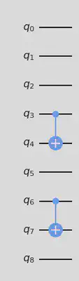
Let us first create a PQC that satisfies both of the constraints $\sum_{p=1}^N x_{1,p}=1$ and $\sum_{v=1}^N x_{1,v}=1$. Recall, here $v$ refers to the vertex and $p$ represents its order in a prospective cycle. Building for a 3 node graph, let us first build the ‘L’ constraint circuit as shown in the paper!

from qiskit import QuantumRegister, ClassicalRegister
from qiskit.circuit import ParameterVector, QuantumCircuit

l_circuit = QuantumCircuit(n**2)
theta = ParameterVector('theta',length=(n-1)*n-1)

# L-Shaped Entangler
l_circuit.ry(theta[0],0)
l_circuit.cx(0,1)
l_circuit.cx(0,3)

l_circuit.barrier()

#W_phi_p
l_circuit.x(1)
l_circuit.ry(theta[1],2)
l_circuit.cz(1,2)
l_circuit.ry(-theta[1],2)
l_circuit.cx(2,1)

#W_phi_v
l_circuit.x(3)
l_circuit.ry(theta[2],6)
l_circuit.cz(3,6)
l_circuit.ry(-theta[2],6)
l_circuit.cx(6,3)

l_circuit.draw("mpl")
Next, now we need to encode the remaining constraints excluding the ones we applied. Since, the constraints for the remaining part are already determined, they can be read in a similar way as the previous problem by applying the corresponding $CNOT$ gates followed by the parametrized $W$ state gates on the qubits mapped variables as shown below!

from qiskit import QuantumRegister, ClassicalRegister
from qiskit.circuit import ParameterVector, QuantumCircuit

r_circuit = QuantumCircuit(n**2)
theta = ParameterVector('theta',length=(n-1)*n-1)

# Two blocks remaining for N = 3
# Block 1 ---------
r_circuit.x(4)
r_circuit.ry(theta[3],5)
r_circuit.cz(4,5)
r_circuit.ry(-theta[3],5)
r_circuit.cx(5,4)


# Block 2 ---------
r_circuit.x(7)
r_circuit.ry(theta[4],8)
r_circuit.cz(7,8)
r_circuit.ry(-theta[4],8)
r_circuit.cx(8,7)

r_circuit.draw("mpl")
One final step before we join the circuits is making the bridge between L-shape and original entangler. We shall construct it as follows:
from qiskit import QuantumRegister, ClassicalRegister
from qiskit.circuit import ParameterVector, QuantumCircuit

bridge_circuit = QuantumCircuit(n**2)
theta = ParameterVector('theta',length=(n-1)*n-1)

bridge_circuit.cx(3,4)
bridge_circuit.cx(6,7)

bridge_circuit.draw(output="mpl")
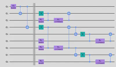
Now we proceed to join all the three circuits as shown in the figure below to complete the routine. We will run the constructed circuit using the RunVQE function which we created in the previous cells to evaluate the result!

from qiskit import QuantumRegister, ClassicalRegister
from qiskit.circuit import ParameterVector, QuantumCircuit

model_2 = QuantumCircuit(n**2)
theta = ParameterVector('theta',length=(n-1)*n-1)

model_2 = l_circuit.compose(bridge_circuit).compose(r_circuit)
model_2.draw("mpl")
Designing for the fourth case - specific PQC satisfying all constraints
I have skipped the implementation of the third case because of it being more or less similar to the previous case.

Now let us consider the final case for the problem. For the fourth PQC, we consider all constraints to completely exclude the infeasible answers in the above image. Thus, the set of the bases of the quantum states includes only feasible answers. We shall now work on an intuition as to how to exclude all the infeasible results. If we see the 2D grid above, based on the constraints we define, the feasible answers can be interpreted in the form of permutation matrices.
Permutation matrix
A permutation matrix is a sqaure matrix that is made up of only 1s and 0s and each row and column have exactly one 1 only. We may know the matrix $I$, which is called the identity matrix. It is a special case of permutation matrices.
Now that we know the definition of a permutation matrix, we can count the number of feasible answers that exist. If n = 2, there are 2 feasible solutions. Below we can check out what these matrices are.
$$ \begin{bmatrix} 1 & 0\ 0 & 1 \end{bmatrix} , \begin{bmatrix} 0 & 1\ 1 & 0 \end{bmatrix} $$
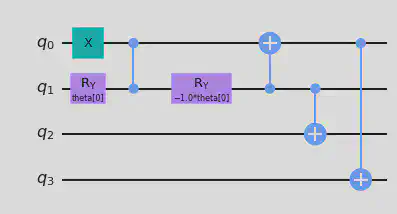
Reflecting these two feasible answers, the circuit below is an example which satisfies all the constraints when n equals 2.
n = 2

perm_circuit = QuantumCircuit(n**2)
theta = ParameterVector('theta',length=(n-1)*n-1)

perm_circuit.x(0)

perm_circuit.ry(theta[0],1)
perm_circuit.cz(0,1)
perm_circuit.ry(-theta[0],1)
perm_circuit.cx(1,0)

perm_circuit.cx(1,2)
perm_circuit.cx(0,3)

perm_circuit.draw("mpl")
Such a PQC for arbitrary $N$ can be constructed in a recursive manner. Because we know the circuit when n = 2, we can construct circuits for the cases $n = 3, 4, … k$. Let’s make the $k \times k$ permutation matrices from the $(k-1) \times (k-1)$ ones.

- Add one row and column which are filled with only zero.
- At the top right, replace 0 to 1.
- Exchange the last column with each column to make a set of permutation matrices.
As the steps above, we can create the desired quantum states as follows:
- Prepare the initialized 2k - 1 qubits, labeled as $q_{k, p’}, p’= 1 … k-1$ and $q_{v, k}, v= 1 … k$.
- Apply a parameterized W state gate to the set of qubits, {$q_{v, k}|v=1 … k$}.
- Apply {$CSWAP_{q_{v’,k}, q_{k,p’}, q_{v’,p’}}|p’=1 … k-1$} for all $v’= 1 … k-1$.
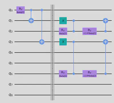
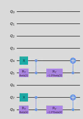
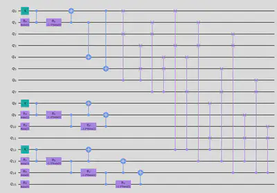
Let’s start on the previous circuit while adding 5 more qubits. Note that CNOT gates’ position is a little different because now $q_2$ in the circuit means $q_{3,1}$.
n = 3
model_3 = QuantumCircuit(n**2)
theta = ParameterVector('theta',length=(n-1)*n//2)

# Build a circuit when n is 2
model_3.x(0)
model_3.ry(theta[0], 1)
model_3.cz(0, 1)
model_3.ry(-theta[0], 1)
model_3.cx(1, 0)
model_3.cx(1, 3)
model_3.cx(0, 4)
model_3.x(6)
model_3.ry(theta[1], 7)
model_3.cz(6, 7)
model_3.ry(-theta[1], 7)
model_3.ry(theta[2], 8)
model_3.cz(7, 8)
model_3.ry(-theta[2], 8)
model_3.cx(7, 6)
model_3.cx(8, 7)
model_3.cswap(6, 2, 0)
model_3.cswap(6, 5, 3)
model_3.cswap(7, 2, 1)
model_3.cswap(7, 5, 4)

model_3.draw("mpl")

# Recursive Approach

n = 3
model_3 = QuantumCircuit(n**2)
theta = ParameterVector('theta',length=(n-1)*n//2)

# Build a circuit when n is 2
model_3.x(0)
model_3.ry(theta[0], 1)
model_3.cz(0, 1)
model_3.ry(-theta[0], 1)
model_3.cx(1, 0)
model_3.cx(1, 3)
model_3.cx(0, 4)

# Apply a parameterized W state gate
model_3.x(6)
model_3.ry(theta[1], 7)
model_3.cz(6, 7)
model_3.ry(-theta[1], 7)
model_3.ry(theta[2], 8)
model_3.cz(7, 8)
model_3.ry(-theta[2], 8)
model_3.cx(7, 6)
model_3.cx(8, 7)

# Apply 4 CSWAP gates
model_3.cswap(6, 2, 0)
model_3.cswap(6, 5, 3)
model_3.cswap(7, 2, 1)
model_3.cswap(7, 5, 4)


model_3.draw("mpl")
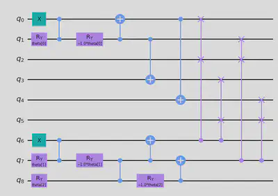
The circuit above represents exactly the superposition of bases of 6 feasible answers. Now we shall call our helper function RunVQE to execute this routine
%%time
# Define optimizer
from qiskit.primitives import Estimator
optimizer = SPSA()

# Define Initial point
np.random.seed(10)
init_3 = np.random.rand((n-1)*n//2) * 2 * np.pi

# Call RunVQE.
with Session(service = service, backend = backend):
    result_m3, mean_m3 = RunVQE(Estimator(), model_3, optimizer, qubitOp, init_3)
CPU times: user 1.18 s, sys: 25.1 ms, total: 1.2 s
Wall time: 1.2 s
optimal_m3 = result_m3.optimal_circuit.measure_all(inplace=False)
%%time
# Compute values
with Session(service=service, backend=backend):
    energy_m3, sampler_result_m3, result_val_m3, result_m3_bitstring = BestBitstring(result=result_m3, optimal_circuit=optimal_m3)
print("Optimal bitstring = ", result_m3_bitstring[7:])
Optimal bitstring =  [0 0 1 0 1 0 1 0 0]
CPU times: user 30 ms, sys: 2.44 ms, total: 32.5 ms
Wall time: 8.56 s
# Compute cost of the obtained result and display result
TSPCost(energy = energy_m3, result_bitstring = result_m3_bitstring[7:], adj_matrix = adj_matrix)
-------------------
Energy: -4751.000000000001
Tsp objective: 129.9999999999991
Feasibility: True
Solution Vector: [2, 1, 0]
Solution Objective: 130.0
-------------------
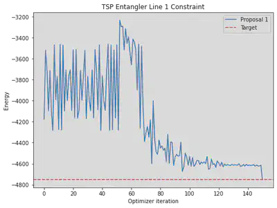
Plot Convergence
# Plot convergence
PlotGraph(mean = [mean,mean_m3], ideal = ideal)
# PlotGraph(mean = [mean,mean_m2,mean_m3], ideal = ideal)
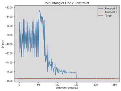
We see a flat lined result close to the ideal result with an ideal simulator because it contains essentially only the feasible solution subspace which converges very fast in an ideal scenario.
Now it’s time to give it another go! Formulate a PQC for a 4 node graph in order to attempt a convergence for a given 4 node graph!
n = 4
num_qubits = n**2

# the target graph
tsp = Tsp.create_random_instance(n, seed=123)

colors = ["tab:red" for node in tsp.graph.nodes]
pos = [tsp.graph.nodes[node]["pos"] for node in tsp.graph.nodes]

draw_graph(tsp.graph, colors, pos)

qp = tsp.to_quadratic_program()
qp2qubo = QuadraticProgramToQubo()
qubo = qp2qubo.convert(qp)
qubitOp_4, _ = qubo.to_ising()
model = QuantumCircuit(n**2)
theta = ParameterVector('theta',length=(n-1)*n//2)

# Build a circuit when n is 3

model.x(0)
model.ry(theta[0], 1)
model.cz(0, 1)
model.ry(-theta[0], 1)
model.cx(1, 0)
model.cx(1, 4)
model.cx(0, 5)

model.x(8)
model.ry(theta[1], 9)
model.cz(8, 9)
model.ry(-theta[1], 9)
model.ry(theta[2], 10)
model.cz(9, 10)
model.ry(-theta[2], 10)
model.cx(9, 8)
model.cx(10, 9)

model.cswap(6, 2, 0)
model.cswap(6, 5, 3)
model.cswap(7, 2, 1)
model.cswap(7, 5, 4)

# Apply a parameterized W state gate
model.x(12)
model.ry(theta[3], 13)
model.cz(12, 13)
model.ry(-theta[3], 13)
model.ry(theta[4], 14)
model.cz(13, 14)
model.ry(-theta[4], 14)
model.ry(theta[5], 15)
model.cz(14, 15)
model.ry(-theta[5], 15)
model.cx(13, 12)
model.cx(14, 13)
model.cx(15, 14)

# Apply CSWAP gates
model.cswap(12, 3, 0)
model.cswap(12, 7, 4)
model.cswap(12, 11, 8)
model.cswap(13, 3, 1)
model.cswap(13, 7, 5)
model.cswap(13, 11, 9)
model.cswap(14, 3, 2)
model.cswap(14, 7, 6)
model.cswap(14, 11, 10)

model.draw("mpl")
%%time
from qiskit.utils import algorithm_globals
from qiskit.primitives import Estimator
algorithm_globals.random_seed = 1024

# Define optimizer
optimizer = SPSA(maxiter=100)

# Define Initial point
np.random.seed(10)
init = np.random.rand((n-1)*n//2) * 2 * np.pi

# Define backend
backend = service.backends(simulator=True)[0]

# Call RunVQE
with Session(service = service, backend = backend):
    result_4, mean = RunVQE(Estimator(), model, optimizer, qubitOp_4, init=init)

# Print result
print(result_4)
{   'aux_operators_evaluated': None,
    'cost_function_evals': 200,
    'eigenvalue': -51498.39338093223,
    'optimal_circuit': <qiskit.circuit.quantumcircuit.QuantumCircuit object at 0x7fc9dd07f970>,
    'optimal_parameters': {   ParameterVectorElement(theta[5]): 2.240446713772086,
                              ParameterVectorElement(theta[3]): 3.758102867479218,
                              ParameterVectorElement(theta[4]): 2.1639129152939685,
                              ParameterVectorElement(theta[1]): 1.5707178278180862,
                              ParameterVectorElement(theta[2]): 4.713181434285074,
                              ParameterVectorElement(theta[0]): 9.758371425063673},
    'optimal_point': array([9.75837143, 1.57071783, 4.71318143, 3.75810287, 2.16391292,
       2.24044671]),
    'optimal_value': -51498.39338093223,
    'optimizer_evals': None,
    'optimizer_result': <qiskit.algorithms.optimizers.optimizer.OptimizerResult object at 0x7fc9dd21af40>,
    'optimizer_time': 23.583685159683228}
CPU times: user 1min 10s, sys: 1min 49s, total: 2min 59s
Wall time: 23.6 s
optimal = result_4.optimal_circuit.measure_all(inplace=False)
%%time
# Compute values
with Session(service=service, backend=backend):
    energy, sampler_result, result_val, bitstring = BestBitstring(result=result_4, optimal_circuit=optimal)
print("Optimal bitstring = ", bitstring)
Optimal bitstring =  [0 0 0 1 0 1 0 0 0 0 1 0 1 0 0 0]
CPU times: user 39.6 ms, sys: 5.59 ms, total: 45.2 ms
Wall time: 33.3 s
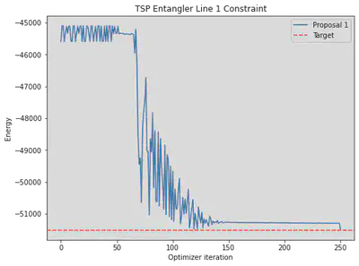
# Plot convergence
ee = NumPyMinimumEigensolver()
result = ee.compute_minimum_eigenvalue(qubitOp_4)
energy_numpy = result.eigenvalue.real

PlotGraph(mean = [mean], ideal = energy_numpy)
Experimental Results
Conclusion
In this implementation and work, I have presented the problem-specific PQCs of the VQE algorithm for the travelling salesman problem. In the PQCs, I have thoroughly discussed the constraints of the problem and have designed circuit to incorporate them. By doing this, it is possible to significantly reduce search spaces. As a result, we can speed up the convergence of the VQE algorithms.
Bibliography
- [1] Solving Combinatorial Optimziation Problems using QAOA
- [2] Max-Cut and Traveling Salesman Problem
- [3] Quantum Bridge Analytics I: A Tutorial on Formulating and Using QUBO Models
- [4] Matsuo, A., Suzuki, Y., & Yamashita, S. Problem-specific parameterized quantum circuits of the VQE algorithm for optimization problems. 2020.
- [5] IBM QISKIT Textbook helped me gain the idea about usage of various functions available in qiskit.
- [6] IBM Quantum Fall Challenge 2022 is what inspired me to take up this project.
- [7] Introduction to Quantum Computing by Qubit by Qubit and IBM was very helpful in helping me understand the core concepts of Quantum Computing which helped me put together this project.
Reflection Questions
-
Was there anything else you would have liked to add to your project if you had more time?
- I would have loved to use PQCs and all the things, I learnt from the implementation of VQE to solve the TSP problem, to solve various other optimization problems speacially the ones observed in Machine Learning and Chemistry, where we optimize some objective function in order to attain higher accuracy and generalizability of our model or try to find the molecular structure with minimum energy level. Additionally, I could have experiment with various Quantum Error Correction techniques and their impact on the results of this Optimization Problem.
-
What challenges did you face? What may you have done differently?
- Setting up the environment, converting the instructions and circuit diagram in the paper to fully functional quantum circuits and figuring out how to fit the pieces together was by far the most challenging task I faced.
- The paper included gates which I haven’t learnt in the course like CSWAP, etc. Hence, it was difficult to understand the working of the Quantum Circuit at first. Although challenging, it was extremely rewarding to finally being able to understand and implement these circuits. Not just for hard-coded number of qubits, but for any N number of qubits!
-
What course concepts does your project connect to and how?
- This project is highly intertwined with the concepts I learnt throughout the course, which includes designing quantum circuit, understanding the high-level working on VQEs and representing the qubit states in mathematical expressions. This high-level understanding helped me substantially to understand the internal working and implementation of these tools.
-
How does this project relate to your interests or career goals?
- I am a Statistics Undergraduate, planning to pursue research in my academic career. This project aligns with my research interests of exploring Quantum Machine Learning and Optimization. I highly believe that the confidence and knowledge I acquired while attempting to work on this project gave me a taste of how research looks in the Quantum Domain. I further intend to explore topics like Quantum Error Correction which I found quite intriguing during the course.
-
How does this project relate to the societal or ethical impact of quantum/AI on the future?
- Being able to solve NP-Hard problem with better and better approximation has always been a chase ever since computers started becoming prevalent. Quantum Computation promises to be very effective in being exponentially faster compared to their classical counterparts. This project is a effort in that direction in showing how Quantum Computation can be leveraged to approximate solutions for these computationally hard problems. In particular, solving the Travelling Salesman Problem has the potential to change the face of logistics and supply chain management to create better optimized travel and delivery routes.
-
What did you most enjoy about this project?
- While working on this project, I gained hands-on knowledge with implementation of Quantum research papers. The most enjoyable thing about this project learn about the new concepts and see the Quantum Circuit run on an actual Quantum Computer to come up with results which have real-life implications. Seeing the results and plots obtained in my experimentation and implementation match with that of the research paper made me ecstatic and confident that my implementation was correct.
Rishi Dey Chowdhury
Master of Statistics
My research interests include Artificial Intelligence, Quant Trading, Deep Learning and their applications in Market Microstructure, Computer Vision and NLP.